Timeseries Clustering using Diffusion Maps
In this blog post we will explore diffusion maps for Timeseries Clustering on the UCI-HAR dataset[1].
Understanding Diffusion maps
Diffusion maps are a nonlinear dimensionality reduction technique that models a dataset as a Markov chain, where the probability of moving from one point to another is based on their similarity(we get this from the diffusion kernel which we explore in this blog). This is done by simulating random walks on the dataset, (called the diffusion process).
Glossary:
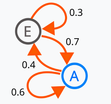
Markov Chain: If you are familiar with Finite State automata this is very similar to that. It is a system that moves between different states step by step, where the next step depends only on the current state (not past history).
 [2]
[2]
Random Walk: It’s a type of Markov Chain where we randomly move from one place to another based on probabilities.
For diffusion maps, the probabilities are based on the distances, closer points have higher transition probability.
Consider n datapoints, we can create a transition matrix P where $P_{ij}$ denotes the probability of sum of all paths going from point $x_i$ to $x_j$ in the dataset X.
This transition probability can be given by the Diffusion kernel, where d(xi, xj) is the DTW distance in case of time series data.
$K_{ij} = \exp \left(-\frac{d(x_i, x_j)^2}{\varepsilon} \right)$
Using the Perron-Frobenius Theorem: Which states that Any matrix M that is positive (aij > 0), column stochastic matrix ($\sum_{i} a_{ij}$ = 1 ∀j)
Hence, We can say that the matrix P gives 1 as the largest eigen value and all other eigen values are <1.
Another thing is if we take $P^t$ then the elements $P_{ij}$ represent the probability of all paths of length t going from $x_i$ to $x_j$
Algorithm taken from [3] which was presented in [4] 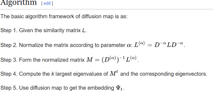
Defining Diffusion Distance between $x_i$ and $x_j$
\[D_{t}(x_{i}, x_{j})^2 = \sum_{k}(|P_{ik}^t - P_{jk}^t|)^2\]Note, we do not need to calculate P to find the diffusion distance It can be shown that,
\[|Y_{i}-Y_{j}|^2 = D_{t}(x_{i}, x_{j})^2\]where $Y_{i} = (P_{i1}^t, P_{i2}^t, …, P_{in}^t).T $
$Y_{i}$ is a vector T represents transpose
If we use diffussion distance in the original dataspace as a measure of similarity then when we project this data in the diffusion/embedding space the similarity is preserved as noted in the above equation.
Note that we can take the first k elements(excluding the 1st eigen vector) from the vector $Y_{i}$ In the below code I have taken k=3
Load the dataset
import pandas as pd
import numpy as np

def load_dataset():
    base_path = 'UCI-HAR Dataset/train/Inertial Signals/'
    signals = [
        'body_acc_x', 'body_acc_y', 'body_acc_z',
        'body_gyro_x', 'body_gyro_y', 'body_gyro_z',
        'total_acc_x', 'total_acc_y', 'total_acc_z'
    ]

    data = [pd.read_csv(f"{base_path}{signal}_train.txt", sep=r"\s+", header=None) for signal in signals]

    x = np.stack(data, axis=1)
    print(x.shape)
    return x

X_train = load_dataset()
(7352, 9, 128)
y_train = pd.read_csv('UCI-HAR Dataset/train/y_train.txt', header=None)
y_train = y_train.values.ravel()
y_train.shape
(7352,)
Pairwise distance matrix(similarity matrix)
This specific implementation for Dimensionality reduction using Diffusion maps is adapted from this.[5]
# Eucledean Pairwise distance matrix
pairwise_eucleadean_dissimilarity_matrix = np.zeros((1000, 1000))
for i in range(X_train[:1000].shape[0]):
    for j in range(X_train[:1000].shape[0]):
        pairwise_eucleadean_dissimilarity_matrix[i][j] = np.linalg.norm(X_train[i] - X_train[j])
from aeon.distances.elastic import dtw_pairwise_distance

pairwise_dtw_dissimilarity_matrix = dtw_pairwise_distance(X_train[:1000], window=25, itakura_max_slope=0.5)
Implementation Note
Note that in step 2 I have used the value of alpha = 1, as this gives the best scores.
pairwise_dtw_dissimilarity_matrix_no_bound.ravel().shape
(1000000,)
import matplotlib.pyplot as plt
import numpy as np
from matplotlib import colors
from matplotlib.ticker import PercentFormatter
N_points = 1000000
n_bins = 20
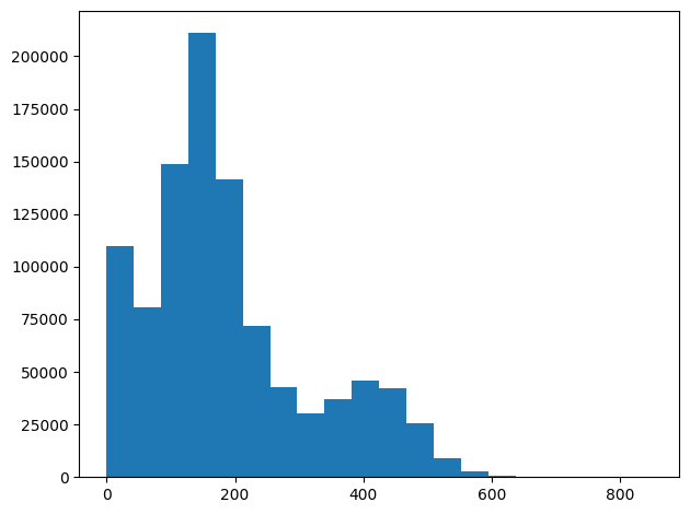
# Plot histogram for distances to see the distribution
fig, axs = plt.subplots(1, 1, sharey=True, tight_layout=True)
axs.hist(pairwise_dtw_dissimilarity_matrix_no_bound.ravel(), bins=n_bins)
plt.show()

sigma_median = np.median(pairwise_dtw_dissimilarity_matrix_no_bound.ravel())
print("Median sigma =", sigma_median)
Median sigma = 158.54597173560018
# kernel matrix
from scipy.linalg import eigh

# similarity_matrix = np.exp(-pairwise_dtw_dissimilarity_matrix) # already squared(see aeon implementation)
similarity_matrix = np.exp(-pairwise_dtw_dissimilarity_matrix_no_bound/sigma_median) # already squared(see aeon implementation)

# dividing by sigma median to normalize the kernel matrix, improves the clustering
# significantly. This is because if dtw_distance was very big then the similarity
# would be very small and vice versa. So, normalizing it makes the similarity
# matrix more consistent.

D = np.diag(similarity_matrix.sum(axis = 1))   # symmetric dose not matter row or column

# P = similarity_matrix/D[:, None]    # markov transition matrix has probablity of going from i to j
# Can parallelize this step using matrix multiplication
P = np.linalg.inv(D) @ similarity_matrix

# symm_P = (P + P.T)/2

eigenvalues, eigenvectors = np.linalg.eig(P)

idx = np.argsort(eigenvalues)[::-1]
eigenvalues = eigenvalues[idx]
eigenvectors = eigenvectors[:, idx]

def compute_diffusion_coords(eigenvectors, eigenvalues, n_components, time=1):
    # Considering random walk with 1 step(focuses on local structure    )
    # Increasing t means diffusion will happen with t steps
    # this smoothens the data and focuses on global structure
    # return eigenvectors @ np.diag(np.exp(-time * eigenvalues))[:, 1:n_components+1]
    # print(eigenvectors.shape, eigenvalues.shape)
    # print(eigenvectors[:, 1:n_components+1].shape, eigenvalues[1:n_components+1].shape)
    # print((eigenvectors[:, 1:n_components+1] * eigenvalues[1:n_components+1]).shape)
    return eigenvectors[:, 1:n_components+1] * (eigenvalues[1:n_components+1]**time)
# without dividing by sigma median
# clustering dosent correspond well with the ground truth labels even though the cluster formed
# are very distinct. This is because the similarity matrix is not normalized and hence the
# kernel matrix is not consistent. This is why the clustering is not good.
import numpy as np
import matplotlib.pyplot as plt
from scipy.spatial.distance import euclidean
from sklearn.cluster import KMeans, DBSCAN
from sklearn.metrics import adjusted_rand_score, silhouette_score
from sklearn.decomposition import PCA
from sklearn.manifold import TSNE
from scipy.linalg import eigh
def clustering_and_evaluation(embedding, true_labels, method='kmeans'):

    if method == 'kmeans':
        k = len(np.unique(true_labels))
        clustering_model = KMeans(n_clusters=k, random_state=42)
    elif method == 'dbscan':
        clustering_model = DBSCAN(eps=0.5, min_samples=5)
    else:
        raise ValueError("Unsupported clustering method")
    print(embedding.shape)
    cluster_labels = clustering_model.fit_predict(embedding)
    ari = adjusted_rand_score(true_labels, cluster_labels)
    sil_score = silhouette_score(embedding, cluster_labels)
    return cluster_labels, ari, sil_score
def flatten_data(X):
    return X.reshape(X.shape[0], -1)

def compute_pca(X, n_components=2):
    pca = PCA(n_components=n_components, random_state=42)
    return pca.fit_transform(X)

def compute_tsne(X, n_components=2):
    tsne = TSNE(n_components=n_components, random_state=42)
    return tsne.fit_transform(X)

activity_labels = {
    1: "WALKING",
    2: "WALKING_UPSTAIRS",
    3: "WALKING_DOWNSTAIRS",
    4: "SITTING",
    5: "STANDING",
    6: "LAYING"
}


def plot_embedding(embedding, labels, title):
    plt.figure(figsize=(8,6))

    unique_labels = np.unique(labels)
    colors = plt.cm.tab10(np.linspace(0, 1, len(unique_labels)))

    for i, label in enumerate(unique_labels):
        idx = labels == label
        plt.scatter(embedding[idx, 0], embedding[idx, 1],
                    label=activity_labels[label], c=[colors[i]], alpha=0.5, edgecolors='k')

    # plt.scatter(embedding[:, 0], embedding[:, 1], c=labels, cmap='viridis', alpha=0.7)
    plt.title(title)
    plt.legend(title="Activities", loc="best", fontsize=10)
    plt.xlabel('Component 1')
    plt.ylabel('Component 2')
    plt.colorbar()
    plt.show()
Clustering in the Diffusion Space
time = 1 seems to be the best choice
print(np.real(eigenvalues))
[ 1.00000000e+00  5.10709410e-01  1.59185685e-01  7.01208713e-02
  5.86290417e-02  5.44986297e-02  4.85806574e-02  3.92711208e-02
  3.77986230e-02  3.31930978e-02  2.97729220e-02  2.57865631e-02
  2.27786946e-02  2.13976380e-02  1.90922118e-02  1.75663302e-02
  1.66536350e-02  1.40842131e-02  1.35790227e-02  1.19211167e-02
  1.16086840e-02  1.11562920e-02  1.08600206e-02  9.72385095e-03
  9.51495420e-03  9.43363561e-03  8.56912266e-03  8.20538175e-03
  8.14241637e-03  7.82629928e-03  7.64774099e-03  7.38961193e-03
  7.06504236e-03  6.98073327e-03  6.77123661e-03  6.40790351e-03
  6.24379808e-03  6.03694588e-03  5.94112224e-03  5.86769252e-03
  5.66030996e-03  5.56448903e-03  5.40347299e-03  5.31873642e-03
  5.21414961e-03  5.05759181e-03  4.95343007e-03  4.81630911e-03
  4.72782975e-03  4.64147118e-03  4.51920316e-03  4.48258315e-03
  4.42358214e-03  4.26102615e-03  4.16472700e-03  4.12950765e-03
  3.96247482e-03  3.86259312e-03  3.82837976e-03  3.76211123e-03
  3.73260031e-03  3.66807578e-03  3.64348223e-03  3.56552681e-03
  3.56026329e-03  3.43267985e-03  3.37909011e-03  3.36672715e-03
  3.27302270e-03  3.23680687e-03  3.16773059e-03  3.10408817e-03
  3.06397069e-03  3.03138408e-03  3.00452696e-03  2.97551334e-03
  2.95723187e-03  2.93684972e-03  2.90183275e-03  2.86672813e-03
  2.83816036e-03  2.81155568e-03  2.73773267e-03  2.69571208e-03
  2.68133966e-03  2.65820747e-03  2.62776718e-03  2.59129062e-03
  2.55013714e-03  2.51589529e-03  2.50247480e-03  2.47691059e-03
  2.44681790e-03  2.43865274e-03  2.40249724e-03  2.37431185e-03
  2.35128644e-03  2.34242248e-03  2.32375054e-03  2.28142475e-03
  2.25709976e-03  2.22304957e-03  2.21753175e-03  2.20340926e-03
  2.16680757e-03  2.15272669e-03  2.14135245e-03  2.11397226e-03
  2.10286320e-03  2.07779145e-03  2.06760631e-03  2.04427276e-03
  2.03653499e-03  2.01300515e-03  2.00833714e-03  1.99015820e-03
  1.97381858e-03  1.95943094e-03  1.92400499e-03  1.91980203e-03
  1.89458045e-03  1.88356126e-03  1.86722968e-03  1.86301944e-03
  1.84355023e-03  1.83144488e-03  1.82159591e-03  1.80664766e-03
  1.79435193e-03  1.77806038e-03  1.77516199e-03  1.76778555e-03
  1.76549510e-03  1.74271721e-03  1.71708027e-03  1.69965991e-03
  1.68604069e-03  1.66608171e-03  1.65802999e-03  1.63120331e-03
  1.62192319e-03  1.60370422e-03  1.59015203e-03  1.58442935e-03
  1.57278482e-03  1.55209864e-03  1.54939003e-03  1.54466671e-03
  1.52236364e-03  1.51738158e-03  1.50390335e-03  1.49057796e-03
  1.47619761e-03  1.46620117e-03  1.46036175e-03  1.45586412e-03
  1.44135426e-03  1.42777023e-03  1.42012626e-03  1.41026170e-03
  1.40284735e-03  1.39221660e-03  1.37757606e-03  1.36509362e-03
  1.36356207e-03  1.35955929e-03  1.34472365e-03  1.32502510e-03
  1.31749659e-03  1.31413357e-03  1.29967211e-03  1.29917865e-03
  1.29131048e-03  1.28652415e-03  1.27771118e-03  1.26414839e-03
  1.25181721e-03  1.24615181e-03  1.23732420e-03  1.22922393e-03
  1.22413875e-03  1.21309564e-03  1.20075808e-03  1.19729051e-03
  1.19376992e-03  1.18223982e-03  1.16390644e-03  1.15443962e-03
  1.15412462e-03  1.14163430e-03  1.13659579e-03  1.12873654e-03
  1.12470319e-03  1.11280514e-03  1.10439152e-03  1.09996243e-03
  1.09831490e-03  1.08615540e-03  1.07240409e-03  1.06621426e-03
  1.06218041e-03  1.04991309e-03  1.04576602e-03  1.03966808e-03
  1.03242318e-03  1.03040500e-03  1.02690463e-03  1.01995355e-03
  1.01210589e-03  1.00352071e-03  9.92817359e-04  9.87770621e-04
  9.79731045e-04  9.72747659e-04  9.70425770e-04  9.65386076e-04
  9.60804740e-04  9.53700662e-04  9.36889949e-04  9.33542713e-04
  9.24616826e-04  9.21945909e-04  9.18334681e-04  9.14679960e-04
  9.09003021e-04  8.99600886e-04  8.95882528e-04  8.90013293e-04
  8.84493909e-04  8.77181298e-04  8.72427695e-04  8.63039083e-04
  8.51736595e-04  8.46708780e-04  8.42421626e-04  8.41322731e-04
  8.30291222e-04  8.27486297e-04  8.18702204e-04  8.15800499e-04
  8.09480469e-04  8.05920072e-04  8.05426402e-04  7.98317758e-04
  7.92791373e-04  7.86876284e-04  7.84988267e-04  7.78936119e-04
  7.64786616e-04  7.61859061e-04  7.58031889e-04  7.51666267e-04
  7.48402329e-04  7.39397643e-04  7.37316735e-04  7.31965725e-04
  7.28944682e-04  7.24094726e-04  7.17022800e-04  7.11501102e-04
  7.05825689e-04  7.00688764e-04  6.97012345e-04  6.95059738e-04
  6.89921896e-04  6.79554942e-04  6.77106768e-04  6.70433499e-04
  6.62112452e-04  6.57887375e-04  6.56108017e-04  6.53119645e-04
  6.50626170e-04  6.43721880e-04  6.41999841e-04  6.35045246e-04
  6.33584103e-04  6.20822915e-04  6.15658813e-04  6.09861806e-04
  6.03807133e-04  6.02455819e-04  5.96881880e-04  5.94635171e-04
  5.86749075e-04  5.83906829e-04  5.79259576e-04  5.74165671e-04
  5.68913964e-04  5.66804944e-04  5.60115659e-04  5.57878091e-04
  5.54698255e-04  5.48934265e-04  5.41973568e-04  5.39153890e-04
  5.37091676e-04  5.32134298e-04  5.29605102e-04  5.28376368e-04
  5.26482405e-04  5.21774777e-04  5.19492716e-04  5.11940118e-04
  5.10972226e-04  5.09470567e-04  5.08100871e-04  5.01810325e-04
  4.98032636e-04  4.92644165e-04  4.88356781e-04  4.86972592e-04
  4.76410288e-04  4.75795174e-04  4.71190876e-04  4.68040204e-04
  4.64095707e-04  4.58830569e-04  4.55500903e-04  4.54000413e-04
  4.49132146e-04  4.46382065e-04  4.42804764e-04  4.39395085e-04
  4.36463374e-04  4.32464221e-04  4.30515069e-04  4.26944536e-04
  4.26610066e-04  4.16412546e-04  4.13552930e-04  4.09797674e-04
  4.06027649e-04  4.02353540e-04  3.98916780e-04  3.97396746e-04
  3.94143846e-04  3.92511064e-04  3.87723342e-04  3.85862525e-04
  3.83563388e-04  3.79663003e-04  3.76026939e-04  3.71517058e-04
  3.70546426e-04  3.64739287e-04  3.61878290e-04  3.58070162e-04
  3.56073562e-04  3.54211846e-04  3.49115628e-04  3.45851139e-04
  3.43557404e-04  3.41285240e-04  3.41074991e-04  3.35569363e-04
  3.32264486e-04  3.24530329e-04  3.21245632e-04  3.20466747e-04
  3.17218073e-04  3.13412803e-04  3.10375641e-04  3.07014007e-04
  3.06239738e-04  3.01719760e-04  2.99305342e-04  2.94827177e-04
  2.92490122e-04  2.91190780e-04  2.87452102e-04  2.84016182e-04
  2.78799734e-04  2.76687924e-04  2.74827637e-04  2.71045285e-04
  2.69956147e-04  2.66110216e-04  2.63899431e-04  2.62265132e-04
  2.58388882e-04  2.56246911e-04  2.54494021e-04  2.52947098e-04
  2.50837078e-04  2.46692408e-04  2.42873958e-04  2.41208650e-04
  2.36723445e-04  2.32578766e-04  2.30870656e-04  2.30190902e-04
  2.29158845e-04  2.25371993e-04  2.19984084e-04  2.16187148e-04
  2.15653103e-04  2.15145001e-04  2.08390601e-04  2.05624180e-04
  2.03809445e-04  2.00904990e-04  1.99403163e-04  1.97001469e-04
  1.95991974e-04  1.90910541e-04  1.89234783e-04  1.87042667e-04
  1.84399575e-04  1.83263592e-04  1.81481261e-04  1.76629083e-04
  1.75170086e-04  1.73944884e-04  1.70407062e-04  1.69581312e-04
  1.65056761e-04  1.64185712e-04  1.61915171e-04  1.59183812e-04
  1.57690417e-04  1.53733448e-04  1.51658368e-04  1.50677381e-04
  1.48312252e-04  1.45343273e-04  1.42962386e-04  1.42615068e-04
  1.41175828e-04  1.39733739e-04  1.38251932e-04  1.36782512e-04
  1.34436868e-04  1.33666370e-04  1.30787235e-04  1.25932063e-04
  1.24002685e-04  1.23114730e-04  1.19489536e-04  1.16161667e-04
  1.15111464e-04  1.11542718e-04  1.09390992e-04  1.08468488e-04
  1.07823474e-04  1.05337194e-04  1.03273646e-04  1.01611555e-04
  1.00254324e-04  9.80551511e-05  9.71271910e-05  9.38818657e-05
  9.25255387e-05  9.15896615e-05  9.06949786e-05  8.97766624e-05
  8.79434127e-05  8.45688169e-05  8.41346948e-05  8.31779481e-05
  8.13806059e-05  7.95793426e-05  7.83264907e-05  7.72154220e-05
  7.49170690e-05  7.46805498e-05  7.23846686e-05  7.08263479e-05
  6.92001326e-05  6.82446658e-05  6.61751750e-05  6.54744056e-05
  6.41273438e-05  6.22130102e-05  6.12452744e-05  5.95731586e-05
  5.94757331e-05  5.77865498e-05  5.69646644e-05  5.57781918e-05
  5.27983690e-05  5.17822167e-05  5.03317516e-05  4.96498558e-05
  4.92413595e-05  4.75191322e-05  4.57193766e-05  4.53682491e-05
  4.46709569e-05  4.34804244e-05  4.18719694e-05  4.10619424e-05
  3.96873459e-05  3.87840648e-05  3.81961159e-05  3.73586893e-05
  3.62415594e-05  3.61769889e-05  3.43380675e-05  3.36479060e-05
  3.24255564e-05  3.19224792e-05  3.14967241e-05  3.06704884e-05
  3.02032524e-05  2.91261574e-05  2.85961541e-05  2.76834160e-05
  2.71772182e-05  2.64799392e-05  2.57750409e-05  2.50360462e-05
  2.48420254e-05  2.39250659e-05  2.31194756e-05  2.22377595e-05
  2.18910693e-05  2.15454633e-05  2.07127257e-05  2.06404360e-05
  2.00369279e-05  1.97047789e-05  1.93578764e-05  1.85604011e-05
  1.81280573e-05  1.75250213e-05  1.69678094e-05  1.66968842e-05
  1.64361440e-05  1.57139675e-05  1.55142518e-05  1.50055262e-05
  1.46361974e-05  1.40399791e-05  1.38998228e-05  1.32865977e-05
  1.31508058e-05  1.27994715e-05  1.23148035e-05  1.21343990e-05
  1.16376463e-05  1.15245950e-05  1.14141336e-05  1.09072775e-05
  1.05764817e-05  1.02458843e-05  1.00450481e-05  9.94656043e-06
  9.57564386e-06  9.41710994e-06  8.78059502e-06  8.41580825e-06
  8.30196323e-06  8.12739462e-06  7.93044609e-06  7.69711938e-06
  7.35686060e-06  7.16315227e-06  7.13995209e-06  6.68402859e-06
  6.66939749e-06  6.55637581e-06  6.23647024e-06  6.03457019e-06
  5.80006317e-06  5.67003279e-06  5.46316229e-06  5.33547111e-06
  5.22067330e-06  5.20455438e-06  4.85438793e-06  4.73427988e-06
  4.60249027e-06  4.52508749e-06  4.43354930e-06  4.27410065e-06
  4.15905177e-06  4.10430296e-06  3.83479942e-06  3.65858533e-06
  3.56805405e-06  3.54520005e-06  3.38741639e-06  3.31540313e-06
  3.18813657e-06  3.11266259e-06  3.01183467e-06  2.98110226e-06
  2.88312703e-06  2.84651978e-06  2.70337266e-06  2.60517359e-06
  2.56933547e-06  2.51870695e-06  2.45865292e-06  2.40223968e-06
  2.32599901e-06  2.22754541e-06  2.15442212e-06  2.09414273e-06
  2.02224771e-06  1.93465656e-06  1.87747980e-06  1.83307285e-06
  1.81669427e-06  1.71653558e-06  1.64732663e-06  1.64143185e-06
  1.59428446e-06  1.55797736e-06  1.47713855e-06  1.42520069e-06
  1.40953459e-06  1.33277260e-06  1.29559559e-06  1.26572359e-06
  1.25279179e-06  1.20072368e-06  1.18338110e-06  1.14811627e-06
  1.13465703e-06  1.11898336e-06  1.10267772e-06  1.05418287e-06
  1.04641466e-06  1.00039559e-06  9.77596992e-07  9.39041796e-07
  9.02847532e-07  8.93969386e-07  8.57167567e-07  8.49855243e-07
  8.26162855e-07  8.02685071e-07  7.90659537e-07  7.48896913e-07
  7.33353299e-07  7.14354879e-07  7.01766161e-07  6.36033594e-07
  6.28795852e-07  6.14877223e-07  6.01496836e-07  5.89753579e-07
  5.65832615e-07  5.57357024e-07  5.46099520e-07  5.21140246e-07
  5.08457165e-07  4.89864423e-07  4.71541857e-07  4.55748513e-07
  4.49313286e-07  4.31959562e-07  4.22610501e-07  4.04233441e-07
  3.83205934e-07  3.79108311e-07  3.58901499e-07  3.51826237e-07
  3.30586083e-07  3.18357617e-07  3.02966485e-07  2.81314611e-07
  2.69605686e-07  2.62601071e-07  2.56495080e-07  2.49140269e-07
  2.41245506e-07  2.30109269e-07  2.17575830e-07  2.12003100e-07
  2.03820327e-07  1.84575904e-07  1.75676442e-07  1.59498234e-07
  1.54582663e-07  1.52968909e-07  1.42441468e-07  1.33895989e-07
  1.21185033e-07  1.12681718e-07  1.04579799e-07  1.00388699e-07
  8.92984647e-08  7.41648923e-08  7.09042543e-08  6.28933400e-08
  4.83677853e-08  4.23788136e-08  2.98114546e-08  2.15230771e-08
  1.39514318e-08 -3.55132245e-09 -1.29652109e-08 -1.44396764e-08
 -2.74744896e-08 -3.13537824e-08 -4.07551948e-08 -5.08029427e-08
 -7.46839598e-08 -8.05856784e-08 -1.00321103e-07 -1.07225825e-07
 -1.17018074e-07 -1.26498325e-07 -1.34519177e-07 -1.45384981e-07
 -1.69740267e-07 -1.78569525e-07 -1.99660493e-07 -2.09051342e-07
 -2.17716446e-07 -2.30037406e-07 -2.50588061e-07 -2.69118076e-07
 -2.77490014e-07 -3.00404546e-07 -3.02618293e-07 -3.08564221e-07
 -3.49598408e-07 -3.71842632e-07 -3.88885037e-07 -3.98330265e-07
 -4.03200744e-07 -4.31050047e-07 -4.44670636e-07 -4.74135444e-07
 -4.79362778e-07 -5.00899742e-07 -5.09213352e-07 -5.49811454e-07
 -5.89219546e-07 -5.98937132e-07 -6.31465469e-07 -6.93206143e-07
 -7.03857757e-07 -7.51823297e-07 -7.55318871e-07 -7.72675371e-07
 -8.27515463e-07 -8.40035440e-07 -8.62082203e-07 -9.06836774e-07
 -9.32550172e-07 -9.87574059e-07 -9.96731273e-07 -1.08925119e-06
 -1.14609606e-06 -1.16183147e-06 -1.20421824e-06 -1.22629159e-06
 -1.28504195e-06 -1.29588188e-06 -1.36604236e-06 -1.42113834e-06
 -1.47376175e-06 -1.52937579e-06 -1.54422281e-06 -1.61766544e-06
 -1.66126660e-06 -1.71422783e-06 -1.78399712e-06 -1.81249285e-06
 -1.91310751e-06 -1.94147010e-06 -2.13470580e-06 -2.16028236e-06
 -2.17790751e-06 -2.25252758e-06 -2.26486529e-06 -2.41338343e-06
 -2.46141623e-06 -2.55915385e-06 -2.70545826e-06 -2.75210013e-06
 -2.86851668e-06 -2.92719181e-06 -2.93717122e-06 -3.06401325e-06
 -3.06538901e-06 -3.14810133e-06 -3.37891828e-06 -3.51169219e-06
 -3.58471246e-06 -3.68293520e-06 -3.72170269e-06 -3.85129844e-06
 -3.99016112e-06 -4.26360862e-06 -4.37029776e-06 -4.49021075e-06
 -4.53410324e-06 -4.79072253e-06 -4.95477391e-06 -5.05160546e-06
 -5.18525630e-06 -5.38648882e-06 -5.47271238e-06 -5.81310591e-06
 -5.89467896e-06 -6.01396593e-06 -6.23520408e-06 -6.57687933e-06
 -6.83135249e-06 -6.90702262e-06 -7.33188363e-06 -7.50229139e-06
 -7.63594786e-06 -7.81088148e-06 -8.13328020e-06 -8.33165602e-06
 -8.73515415e-06 -8.83965752e-06 -9.25033304e-06 -9.43860489e-06
 -9.75449965e-06 -1.02515328e-05 -1.07747105e-05 -1.08824938e-05
 -1.11468606e-05 -1.17545826e-05 -1.18120128e-05 -1.22131421e-05
 -1.25013162e-05 -1.27246058e-05 -1.31138448e-05 -1.36073539e-05
 -1.36804538e-05 -1.41933676e-05 -1.49178159e-05 -1.55249091e-05
 -1.57126545e-05 -1.61433430e-05 -1.64270744e-05 -1.72518084e-05
 -1.74993666e-05 -1.83045590e-05 -1.84394372e-05 -1.92524929e-05
 -1.96471338e-05 -2.04551783e-05 -2.13336381e-05 -2.16518400e-05
 -2.19955019e-05 -2.27259352e-05 -2.31384169e-05 -2.32736399e-05
 -2.43675078e-05 -2.49559090e-05 -2.56176598e-05 -2.65694920e-05
 -2.80834098e-05 -2.91019595e-05 -2.95807291e-05 -3.09516043e-05
 -3.13676083e-05 -3.26782550e-05 -3.33072444e-05 -3.37965291e-05
 -3.48354191e-05 -3.54976891e-05 -3.59551656e-05 -3.79289384e-05
 -3.82612335e-05 -3.99713558e-05 -4.02799452e-05 -4.21590239e-05
 -4.33106322e-05 -4.36325641e-05 -4.54878565e-05 -4.67361806e-05
 -4.77399583e-05 -4.85025919e-05 -5.02226432e-05 -5.11691454e-05
 -5.23048053e-05 -5.36637994e-05 -5.38429483e-05 -5.53412696e-05
 -5.74444800e-05 -5.83480094e-05 -6.09756452e-05 -6.13672828e-05
 -6.19787634e-05 -6.54150709e-05 -6.64247586e-05 -6.96705860e-05
 -7.05438131e-05 -7.18830363e-05 -7.31887443e-05 -7.47536897e-05
 -7.72765370e-05 -7.97472524e-05 -8.05480594e-05 -8.33843432e-05
 -8.72553514e-05 -8.75625885e-05 -8.83931544e-05 -8.99506891e-05
 -9.21368423e-05 -9.48979200e-05 -9.62483789e-05 -1.00173502e-04
 -1.00783595e-04 -1.06938480e-04 -1.07663249e-04 -1.12996039e-04
 -1.13904353e-04 -1.16255392e-04 -1.22187364e-04 -1.25488716e-04
 -1.29378411e-04 -1.30044770e-04 -1.31143286e-04 -1.37959709e-04
 -1.38336957e-04 -1.43838648e-04 -1.45091590e-04 -1.49741738e-04
 -1.52165997e-04 -1.52534178e-04 -1.58946056e-04 -1.60344186e-04
 -1.63625234e-04 -1.70051395e-04 -1.70140441e-04 -1.75953024e-04
 -1.78025198e-04 -1.86868424e-04 -1.88434889e-04 -1.94396414e-04
 -1.96397425e-04 -2.01461181e-04 -2.06652935e-04 -2.14448684e-04
 -2.19574888e-04 -2.22855400e-04 -2.26136279e-04 -2.29423149e-04
 -2.34094480e-04 -2.41331263e-04 -2.41967879e-04 -2.46913443e-04
 -2.59476813e-04 -2.62586369e-04 -2.68169548e-04 -2.70463546e-04
 -2.73883180e-04 -2.80459508e-04 -2.81164381e-04 -2.88887523e-04
 -2.91253532e-04 -2.97077543e-04 -3.02490301e-04 -3.14707664e-04
 -3.20049185e-04 -3.23694074e-04 -3.27221256e-04 -3.37580632e-04
 -3.41044813e-04 -3.49281294e-04 -3.53961769e-04 -3.70598918e-04
 -3.74719858e-04 -3.82762378e-04 -3.97801485e-04 -4.10872473e-04
 -4.14257890e-04 -4.28277389e-04 -4.31357223e-04 -4.41364162e-04
 -4.51810226e-04 -4.66623564e-04 -4.89619508e-04 -5.01584603e-04
 -5.04172163e-04 -5.26958620e-04 -5.29547285e-04 -5.38314270e-04
 -5.58170466e-04 -5.77745596e-04 -6.09281269e-04 -6.29008754e-04
 -6.46959678e-04 -6.78808685e-04 -7.25500692e-04 -7.49969159e-04
 -7.79530246e-04 -8.24572453e-04 -9.13128855e-04 -9.38643690e-04
 -1.01540132e-03 -1.07239434e-03 -1.24240698e-03 -1.39743597e-03
 -1.42494513e-03 -1.71126767e-03 -2.08141929e-03 -2.36880133e-03]
plt.plot(np.real(eigenvalues), 'o-')
plt.title("Eigenvalues of the Markov transition matrix(sorted in descending order)")
plt.xlabel("Index")
plt.ylabel("Eigenvalue")
plt.show()

# We pass the eigenvectors and eigenvalues to the function to compute the diffusion coordinates
# The function returns the diffusion coordinates, by ignoring the first eigenvalue and eigenvector
# The first eigenvalue and eigenvector are ignored because they correspond to the trivial solution

diffusion_coords = np.real(compute_diffusion_coords(eigenvectors, eigenvalues, n_components=3 , time=1))
print("Clustering in diffusion space using KMeans...")
cluster_labels_diff, ari_diff, sil_diff = clustering_and_evaluation(diffusion_coords, y_train[:1000], method='kmeans')
print("Diffusion Map - ARI:", ari_diff, "Silhouette Score:", sil_diff)
Clustering in diffusion space using KMeans...
(1000, 3)
Diffusion Map - ARI: 0.4782825147753031 Silhouette Score: 0.6138027690504942
diffusion_coords_temp = np.real(compute_diffusion_coords(eigenvectors, eigenvalues, n_components=3 , time=8))
print("Clustering in diffusion space using KMeans...")
cluster_labels_diff, ari_diff, sil_diff = clustering_and_evaluation(diffusion_coords_temp, y_train[:1000], method='kmeans')
print("Diffusion Map - ARI:", ari_diff, "Silhouette Score:", sil_diff)
Clustering in diffusion space using KMeans...
(1000, 3)
Diffusion Map - ARI: 0.25297020131276876 Silhouette Score: 0.686669312351343
diffusion_coords_temp = np.real(compute_diffusion_coords(eigenvectors, eigenvalues, n_components=3 , time=50))
print("Clustering in diffusion space using KMeans...")
cluster_labels_diff, ari_diff, sil_diff = clustering_and_evaluation(diffusion_coords_temp, y_train[:1000], method='kmeans')
print("Diffusion Map - ARI:", ari_diff, "Silhouette Score:", sil_diff)
Clustering in diffusion space using KMeans...
(1000, 3)
Diffusion Map - ARI: 0.25297020131276876 Silhouette Score: 0.686669476517941
Visualization and Interpretation
# Plot the diffusion map embedding (using the first two diffusion coordinates)
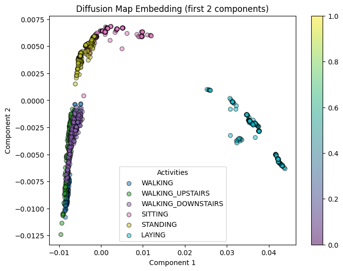
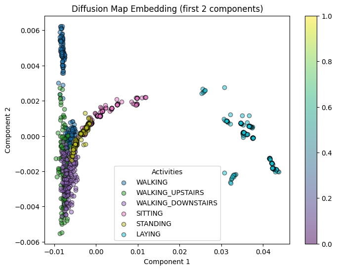
plot_embedding(diffusion_coords[:, :2], y_train[:1000], "Diffusion Map Embedding (first 2 components)")
plot_embedding(diffusion_coords[:, [0, 2]], y_train[:1000], "Diffusion Map Embedding (first and 2nd components)")
X_flat = flatten_data(X_train[:1000])
print("Clustering in raw feature space...")
cluster_labels_raw, ari_raw, sil_raw = clustering_and_evaluation(X_flat, y_train[:1000], method='kmeans')
print("Raw Feature Space - ARI:", ari_raw, "Silhouette Score:", sil_raw)
Clustering in raw feature space...
(1000, 1152)
Raw Feature Space - ARI: 0.2968409437567964 Silhouette Score: 0.13039108175504283
# PCA embedding
pca_coords = compute_pca(X_flat, n_components=3)
print("Clustering in PCA space...")
cluster_labels_pca, ari_pca, sil_pca = clustering_and_evaluation(pca_coords, y_train[:1000], method='kmeans')
print("PCA - ARI:", ari_pca, "Silhouette Score:", sil_pca)
Clustering in PCA space...
(1000, 3)
PCA - ARI: 0.39081158060003784 Silhouette Score: 0.45552093767594737
# t-SNE embedding
tsne_coords = compute_tsne(X_flat, n_components=3)
print("Clustering in t-SNE space...")
cluster_labels_tsne, ari_tsne, sil_tsne = clustering_and_evaluation(tsne_coords, y_train[:1000], method='kmeans')
print("t-SNE - ARI:", ari_tsne, "Silhouette Score:", sil_tsne)
Clustering in t-SNE space...
(1000, 3)
t-SNE - ARI: 0.25734057971635116 Silhouette Score: 0.30087483
# Plot the alternative embeddings
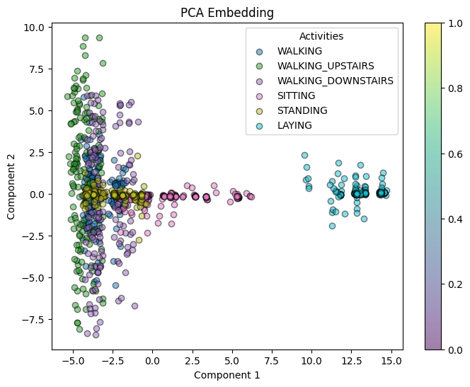
plot_embedding(pca_coords[:, :2], y_train[:1000], "PCA Embedding")
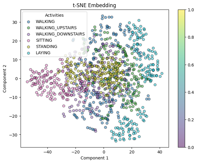
plot_embedding(tsne_coords, y_train[:1000], "t-SNE Embedding")
Observations
Adjusted Rand Index (ARI):
ARI measures how well the clustering results match the known ground truth labels. Here, diffusion maps (ARI ≈ 0.47) outperforms the other methods, meaning that clusters obtained in the diffusion space align best with the activity labels.
PCA (ARI ≈ 0.39) Raw feature space (ARI ≈ 0.297) t-SNE (ARI ≈ 0.257)
This suggests that, in terms of matching the provided labels, diffusion maps produces clusters that most closely reflect the expected classes.
Silhouette Score:
The silhouette score reflects the quality of the clustering, how well-separated and compact the clusters are.
Diffusion maps dominate in this respect with a high silhouette score of 0.688, indicating that within the diffusion space, the clusters are very well-defined and separated.
PCA also shows good separation 0.456, followed by t-SNE 0.300, and raw features shows 0.130.
TODO: # Add legend/labels in the plots
Conclusion: Why diffusion maps perform well for timeseries data/
Capturing Non Linear Manifolds
Diffusion maps work by constructing a Markov process over the data points, where the transition probabilities reflect local similarities(as dtw is a local similarity). This process uncovers the complex nonlinearity of the underlying data manifold(manifold learning).
For time-series data, which often lie on complex, nonlinear manifolds, this means that the essential complex structures(such as temporal correlations) are preserved in the lower-dimensional space after the embedding.
Comparison with Other Techniques
PCA: PCA is a linear dimensionality reduction technique, due to this it can fail to capture the complex, nonlinear structures in the data, for timeseries data with multiple dimensions this is often the case. The slightly lower ARI (≈ 0.39) and silhouette score (≈ 0.456) suggest that PCA does not separate the classes as effectively.
t-SNE: t-SNE is good at preserving local structure but can sometimes distort the global relationships between clusters. Its lower ARI (≈ 0.257) and silhouette score (≈ 0.300) imply that while it can reveal local groupings, it might not be as effective at maintaining the overall cluster structure in the context of time-series.
Raw Feature Space: Clustering in the raw feature space (ARI ≈ 0.297 and silhouette ≈ 0.130) dont form very nice clusters due to high dimensionality and noise, making it harder to uncover the inherent temporal patterns(complex non-linear structures).
Explorative
References Used:
[1]“UCI Machine Learning Repository,” archive.ics.uci.edu. https://archive.ics.uci.edu/dataset/240/human+activity+recognition+using+smartphones
[2] Wikipedia Contributors, “Markov chain,” Wikipedia, Dec. 13, 2019. https://en.wikipedia.org/wiki/Markov_chain
[3] Wikipedia Contributors, “Diffusion map,” Wikipedia, Jan. 03, 2025.
[4] Coifman, R.R.; Lafon, S; Lee, A B; Maggioni, M; Nadler, B; Warner, F; Zucker, S W (2005).
[5] NPTEL IIT Guwahati, “Lec 49: Diffusion maps,” YouTube, Mar. 31, 2022. https://www.youtube.com/watch?v=SaqJ8x4vQ6U (accessed Mar. 25, 2025).
Enjoy Reading This Article?
Here are some more articles you might like to read next: